This tutorial goes over some basic commands and functions for reading in an preparing network data for analysis in R. I will make use of the statnet R package for network analysis. I will provide four examples with different types of data where I take it from its raw form and prepare it for further plotting and analysis using the statnet package. In all cases, I will simulate the data I use for the example, to make it easier to distribute this code, however, the last example will read the simulated data out to .csv files so that I can illustrate reading it back in. The four examples will cover:

1. Preparing an unweighted sociomatrix (adjacency matrix) with accompanying node-level covariates for analysis.
2. Preparing a unweighted edgelist with accompanying node-level covariates for analysis, and then incorporating edge weights into the network object.
3. Preparing an weighted sociomatrix (adjacency matrix) with accompanying node-level covariates for analysis.
4. Preparing a messy unweighted edgelist with multiple receivers for each sender and missing observations from the node accompanying node level dataset for analysis. This example will also cover reading in data from .csv files and will provide a flexible function for making sure that edgelists and node-level datasets conform to each other.

I will also be illustrating different plotting options using the plot.network() function in the network package, which itself is part of the statnet package. While I will be illustrating several options for this function, there are many more than I can cover here. Check out this page for more of a description of the options available for plotting networks using package network. Finally, the last section will provide a function for checking the integrity of your resulting network object by printing out a list of randomly selected edges that you can confirm exist in your source data.

Preliminaries

The first thing we should do is make sure we install the statnet package and all of its dependencies:

install.packages("statnet", dependencies = TRUE) 

First we will take care of some preliminaries before we get started with our example

# Remove everything in our workspace so we can start with a clean slate:
rm(list = ls())
# Set our working directory (for me this is just my desktop)
setwd("~/Desktop")

Now we will want to load in the statnet package:

library(statnet)

Finally we will want to make sure that we set the system seed, which will allow us to replicate our results:

set.seed(12345)

Now we are ready to get down to business! I will cover four different examples of reading in a preparing network data for analysis in the sections below.

Sociomatrix Example

The first example will cover simulating and then reading a 10x10 sociomatrix into a network object using the network package in R.

Simulating The Network

We begin by specifying the number of nodes in the network:

num_nodes <- 10

We can then generate a binary sociomatrix using the matrix() function included in base R:

my_sociomatrix <- matrix(round(runif(num_nodes*num_nodes)), # edge values
                         nrow = num_nodes, #nrow must be same as ncol
                         ncol = num_nodes)

Now we make sure that there are no self-edges in the network. In most cases, we do not expect nodes to form ties to themselves so this is a sensible thing to check for in any sociomatrix:

diag(my_sociomatrix) <- 0

Creating A Network Object

Now we can create a network object using the as.network() function with the following arguments:

net <- as.network(x = my_sociomatrix, # the network object
                  directed = TRUE, # specify whether the network is directed
                  loops = FALSE, # do we allow self ties (should not allow them)
                  matrix.type = "adjacency" # the type of input
                  )

If we want to add in vertex level attributes, we will need to make sure that there are the same number of these attributes as nodes in our network.

Lets add in some made up node names.

network.vertex.names(net) <- LETTERS[1:10]

These could also be entered by hand if one is working with a relatively small network, as in the following example:

network.vertex.names(net) <- c("Susan","Rachel","Angela","Carly","Stephanie","Tom","Mike","Tony","Matt","Steven")

We can then generate and add in a categorical node level variable called "Gender" in the following manner:

# Create the variable
gender <- c(rep("Female",num_nodes/2),rep("Male",num_nodes/2))
# Take a look at our variable
print(gender)
# Add it to the network object
set.vertex.attribute(net, # the name of the network object
                     "Gender", # the name we want to reference the variable by in that object
                     gender # the value we are giving that variable
                     ) 

We can also add in a numeric node level variable called "Age" in a similar manner:

age <- round(rnorm(num_nodes,20,3))
set.vertex.attribute(net,"Age",age)

Now we can take another look at a summary of the network object to make sure everything is added in correctly.

summary.network(net, # the network we want to look at
                print.adj = FALSE # if TRUE then this will print out the whole adjacency matrix.
                )

Plotting The Network

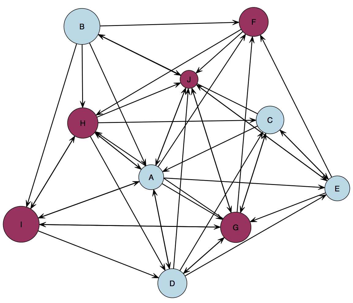
Visualizing a network is always a good place to start before moving on to statistical analyses or further descriptive statistics. It can also often reveal coding errors or things that may have gone wrong in data collection. We also want these plots to look pretty so we can stick them in our journal articles. First, we are going to come up with colors based on the node attribute "Gender":

node_colors <- rep("",num_nodes)
for(i in 1:num_nodes){
  if(get.node.attr(net,"Gender")[i] == "Female"){
    node_colors[i] <- "lightblue"
  }else{
    node_colors[i] <- "maroon"
  }
}
print(node_colors)

Now we can plot our network to a pdf file. Note that this will save the picture directly to a pdf and will not display it anywhere on our screen by default. The file will automatically be saved in our current working directory unless a different directory is specified. We will need to run the entire block of code in order for the pdf file to be finalized and viewable:

pdf("Network_Plot_1.pdf", # name of pdf (need to include .pdf)
    width = 10, # width of resulting pdf in inches
    height = 10 # height of resulting pdf in inches
    ) 
plot.network(net, # our network object
             vertex.col = node_colors, # color nodes by gender
             vertex.cex = (age)/5, # size nodes by their age
             displaylabels = T, # show the node names
             label.pos = 5 # display the names directly over nodes
             )
dev.off() # finishes plotting and finalizes pdf

Now we can go look for the plot in our working directory. If you cannot find it, you can always use the:

getwd()

function to find out where the file was saved. You should end up with a network that looks something like this, with either letters or actual names as the node names:

Edgelist Example

The second example will cover simulating and then reading a edgelist with 80 edges and 40 nodes into a network object using the network package in R.

Simulating The Network

We begin by setting the number of nodes and edges for this example:

num_nodes <- 40
num_edges <- 80

next we can generate node names using the paste function as follows:

node_names <- rep("",num_nodes)
for(i in 1:num_nodes){
  node_names[i] <- paste("person",i,sep = "_")
}
print(node_names)

Now we can create a blank edgelist with spaces for 80 edges which we will populate with names we generated above:

edgelist <- matrix("",nrow= num_edges,ncol = 2)

The following loop will now populate the rows with edge pairs which consist of the name of a sender and the name of a receiver:

for(i in 1:num_edges){
  edgelist[i,] <- sample(x= node_names, # the names we want to sample from
                         size = 2, # sender and receiver
                         replace = FALSE # we do not allow self edges
                         ) 
}
print(edgelist)

Creating A Network Object

Now we are going to initialize a network with the right number of nodes. This step is important because we may have isolates in our network and so the edgelist will not contain any information about them. By ensuring that we represent all nodes first, we avoid inadvertently leaving some out.

net2 <- network.initialize(num_nodes)

Next we will add in the node names so we can match up out edgelist to the nodes in our network object.

network.vertex.names(net2) <- node_names

Now we add in edges from the edgelist to the network object by using the following syntax:

net2[as.matrix(edgelist)] <- 1

we can create an income vertex attribute as follows:

income <- round(rnorm(num_nodes,mean = 50000,sd = 20000))
set.vertex.attribute(net2,"Income",income)

Now lets take a look at our network object using the summary() function to make sure everything looks good:

summary.network(net2,print.adj = FALSE)

We may want to add in edge weights by using the set.edge.value function. Fortunately this is pretty straightforward:

edge_weights <- round(runif(num_edges,min = 1,max = 5))
set.edge.value(net2,"trust",edge_weights)

If necessary, we can get the (binary) adjacency matrix relatively easily now by accessing it from the network object. It is often the case that data may be provided as an edgelist simply because it is compact or easier to collect, but we may want a sociomatrix for some other purpose and this is an easy way to get one without writing the script to convert between the two representations ourselves.

adjacency_matrix_2 <- net2[,]

Plotting The Network

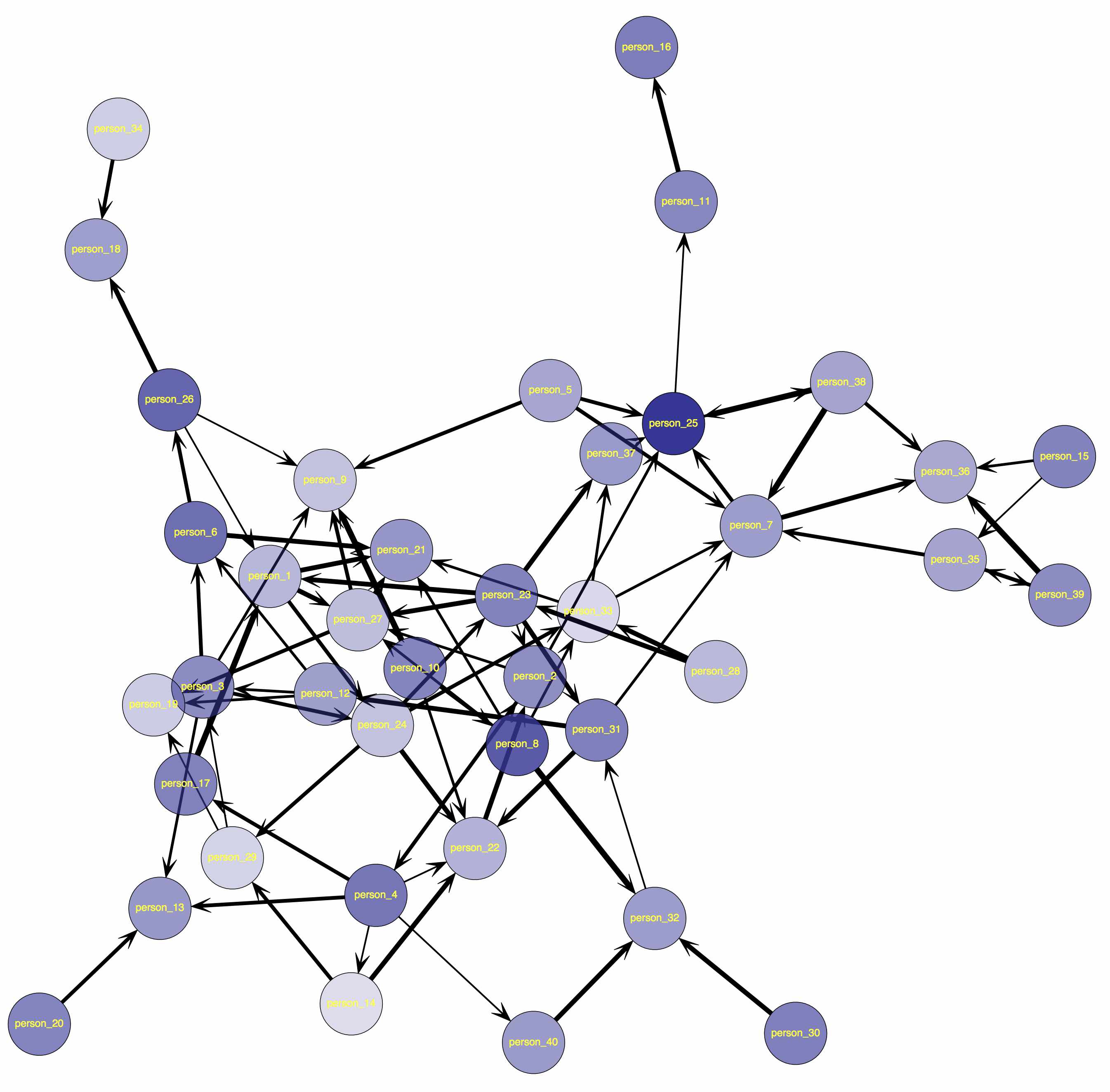
Here we are going to color nodes darker based on how much money they have. Getting the number of nodes in the network directly from the network object (this helps to prevent screw-ups) can be accomplished this way and is nice if we do not know the number off the top of our heads:

num_nodes <- length(net2$val)

We will need to create a blank vector to populate with color names

node_colors <- rep("",num_nodes)

To correctly shade our nodes, we will need to get the maximum income of any node:

maximum <- max(get.node.attr(net2,"Income"))

Now we can loop over each node in the network to calculate how dark they are based on their relative income:

for(i in 1:num_nodes){
  #' Calculate the intensity of the node color depending on the person's 
  #' relative income. 
  intensity <- round((get.node.attr(net2,"Income")[i]/maximum)*255)
  node_colors[i] <- rgb(red = 51, # the proportion of red
                        green = 51, # the proportion of green
                        blue = 153, # the proportion of blue
                        alpha = intensity, # the intensity of the color
                        max = 255 # the maximum possible intensity
                        ) 
}

With the node colors generate, we can now plot our network:

pdf("Network_Plot_2.pdf", # name of pdf (need to include .pdf)
    width = 20, # width of resulting pdf in inches
    height = 20 # height of resulting pdf in inches
) 
plot.network(net2, 
             vertex.col = node_colors, # color nodes by gender
             vertex.cex = 3, # set node size to a fixed value
             displaylabels = T, # show the node names
             label.pos = 5, # display the names directly over nodes
             label.col = "yellow", # the color of node lables
             edge.lwd = get.edge.value(net2,"trust") # edge width based on trust
)
dev.off() # finishes plotting and finalizes pdf

Now we can go look for the plot in our working directory. If you cannot find it, you can always use the:

getwd()

function to find out where the file was saved. You should end up with a network that looks something like this:

Weighted Sociomatrix Example

The third example will cover simulating and then reading a 100x100 weighted sociomatrix into a network object using the network package in R.

Simulating The Network

Again we will create an example sociomatrix, and start by specifying the number of nodes:

num_nodes <- 100

Now we generate random edge values. This bit of code is pretty complicated but essentially we are multiplying edge values against a binary indicator of whether there is an edge at all. This bit of code is not essential to fully understand but can be fun to mess with:

edge_values <- round(runif(n = num_nodes*num_nodes , min = 1, max = 100))*round(runif(n = num_nodes*num_nodes, min = 0, max = .51))

Now we create the sociomatrix as follows:

my_sociomatrix2 <- matrix(edge_values, nrow = 100, ncol = 100)

Again we make sure there are no self-edges:

diag(my_sociomatrix2) <- 0

Now we can create a network object:

net3 <- as.network(x = my_sociomatrix2, # the network object
                  directed = TRUE, # specify whether the network is directed
                  loops = FALSE, # do we allow self ties (should not allow them)
                  matrix.type = "adjacency" # the type of input
)

While we are at it, we can set a node-level attribute called "Size":

size <- round(rnorm(num_nodes,100,10))
set.vertex.attribute(net3,"Size",size)

Now again we can set the edge values and call them "Weights" by simply using the network as the weights:

set.edge.value(net3,"Weight",edge_values)

It is always a good idea to check out a summary of our network to make sure everything looks good.

summary.network(net3,print.adj = FALSE)

Plotting The Network

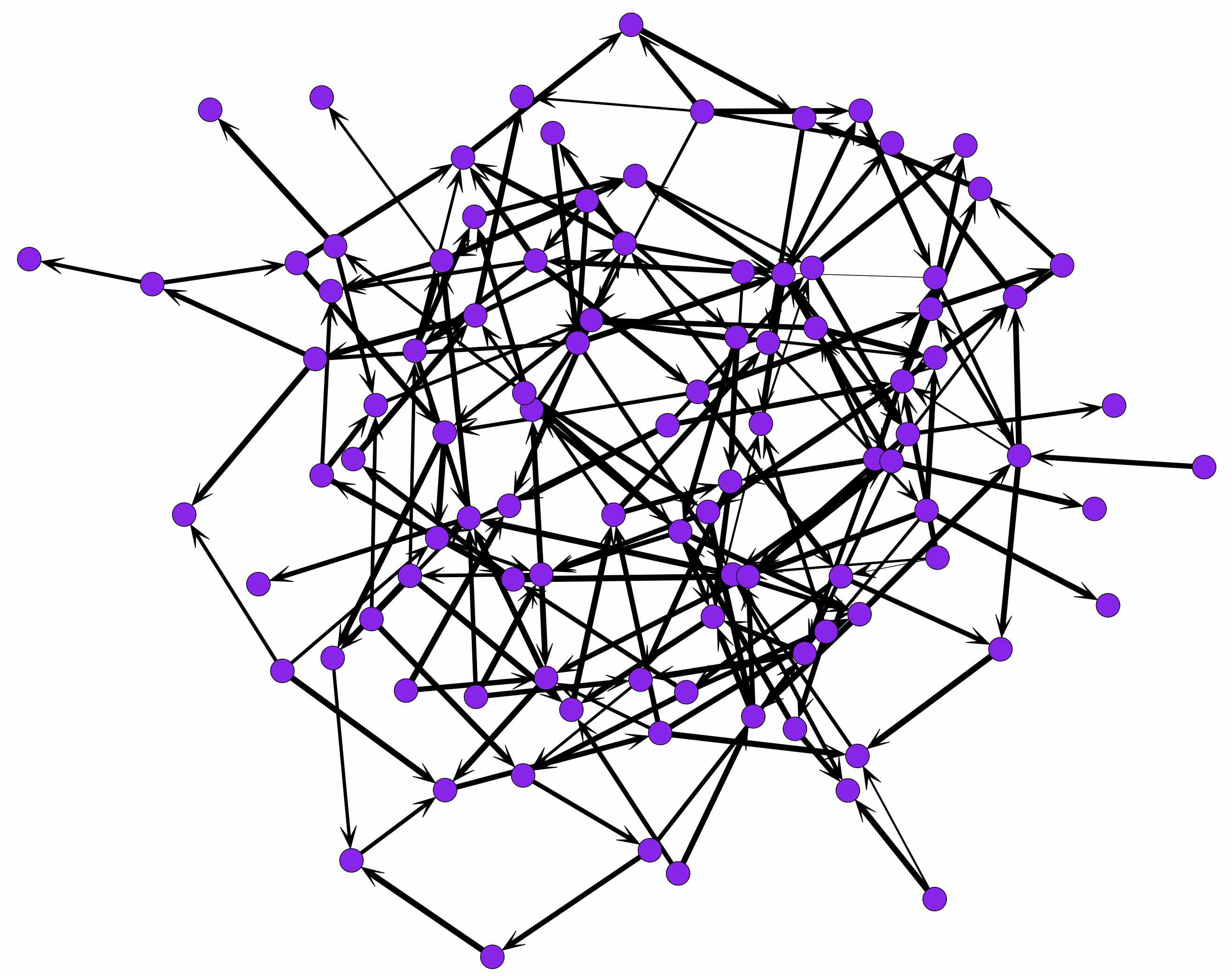
Now we can plot our network (keeping things simple)

pdf("Network_Plot_3.pdf", # name of pdf (need to include .pdf)
    width = 20, # width of resulting pdf in inches
    height = 20 # height of resulting pdf in inches
) 
plot.network(net3, 
             vertex.col = "purple", #just one color
             displaylabels = F, # no node names
             edge.lwd = log(get.edge.value(net3,"Weight")) # edge width
)
dev.off() # finishes plotting and finalizes pdf

Now we can go look for the plot in our working directory. You should end up with a network that looks something like this:

Reading in Real World Data: An edge list with multiple receivers per sender.

You may encounter data where you have one row in your dataset for each sender but multiple receivers (perhaps for campaign contribution data). This example will go over an approach to reading this data into R and turning it into a network object. I will be generating some fake relational and node level data, saving it to .csv files and then reading it in and cleaning it up to provide a full example.

Simulating The Network

We start by specifying the number of nodes we want to use.

num_nodes <- 100

We are going to use the randomNames package to generate some realistic random names for our nodes.

install.packages("randomNames",dependencies = T)
library(randomNames)

Now we will generate a vector of random names:

node_names <- randomNames(num_nodes,name.order = "first.last",name.sep = "_")

Here it is important to make sure we have num_nodes unique names as there is no option to prevent resampling of names using this function.

length(unique(node_names)) == num_nodes

We are going to create a matrix with one row for each potential sender and then an unspecified number of receivers for each sender. To do so, we will need to over-allocate our initial matrix as follows:

relational_information <- matrix(NA,nrow = num_nodes,ncol = num_nodes)

Now we can populated the receiver matrix using a Poisson Process as follows. Again it is not essential for you to get every line of code:

max_receivers <- 0
for(i in 1:num_nodes){
  num_receivers <- min(rpois(n = 1, lambda =2),num_nodes)
  # If there are any recievers for this sender
  if(num_receivers > 0){
    receivers <- sample(x = node_names[-i], size = num_receivers, replace = F)
    relational_information[i,1:num_receivers] <- receivers
  }
  # Keep track on the maximum number of receivers
  if(num_receivers > max_receivers){
    max_receivers <- num_receivers 
  }
}

Now we can put together the sender and receiver information into an extended edgelist.

relational_information <- cbind(node_names,relational_information[,1:max_receivers])

Lets take a look at our fake data using the head function which will only show us the first 4-6 rows of our data

head(relational_information)

Now lets make up some fake node level data:

ages <- round(rnorm(n = num_nodes, mean = 40, sd = 5))
genders <- sample(c("Male","Female"),size = num_nodes, replace = T)
node_level_data <- cbind(node_names,ages,genders)

Uh Oh! We are going randomly scramble the rows and lose some of our data. The point of this exercise is that in real life we may not be able to get node level information for all of the possible nodes in the network we collect, and this data may not be a in a clean format, so I am going to show you how to deal with this. In this case, we are going to lose 10 observations.

node_level_data <- node_level_data[sample(x = 1:num_nodes, size = num_nodes-10),]

Now we can write this data to .csv files:

write.table(x = node_level_data, 
            file = "node_level_data.csv",
            sep = ",",
            row.names = F)
write.table(x = relational_information, 
            file = "relational_information.csv",
            sep = ",",
            row.names = F)

Creating A Network Object

Now lets read everything back in and forget how we actually generated the data. We can start by clearing our working directory:

rm(list = ls())

Then read in the edge matrix and node level covariates:

edge_matrix <- read.csv(file = "relational_information.csv",
                        sep = ",",
                        stringsAsFactors = F, # Always include this argument!
                        header = T)
node_covariates <- read.csv(file = "node_level_data.csv",
                            sep = ",",
                            stringsAsFactors = F, # Always include this argument!
                            header = T)

First check to see if we have the same number of nodes in our two datasets:

nrow(edge_matrix) == nrow(node_covariates)

Ok so in general, we will want to only use those node for which we actually have node level covariates available for in order to avoid tricky situations where some of our data is missing. However, we need to be really careful that those nodes for which we do not have all of the information are missing at random and not because of some systematic flaw in our data collection procedure. I am going to define a function that will make these two objects (or a vanilla edgelist and a set of node level covariates) match up to each other. This function will assume that if there are more nodes in our node level dataset, that these are isolates. If multiple receivers are provided for each sender, this function will automatically turn the resulting dataset into an edgelist os that it can be read into a network object using the statnet package. This function currently does not handle weighted data.

Process_Node_and_Relational_Data <- function(node_level_data,
                                             relational_data,
                                             node_id_column = 1
                                             ){
  #get our node ids
  node_ids <- node_level_data[,node_id_column]
  #remove any missing or blank entries
  to_remove <- which(node_ids == "" | is.na(node_ids))
  if(length(to_remove) > 0){
    node_ids <- node_ids[-to_remove]
    node_level_data <- node_level_data[-to_remove,]
  }
  # Allocate a blank edgelist to return
  edgelist <- NULL
  # Loop over rows to check them
  for(i in 1:length(relational_data[,1])){
    # Check to see if the sender is in the dataset
    if(length(which(node_ids == relational_data[i,1]) > 0)){
      #' If we have a valid sender, check to see if there is a valid reciever 
      #' and add them to the dataset if they are valid as well for each 
      #' receiver
      for(j in 2:ncol(relational_data)){
        if(!is.na(relational_data[i,j])){
          if(length(which(node_ids == relational_data[i,j]) > 0)){
            edge <- c(relational_data[i,1],relational_data[i,j])
            edgelist <- rbind(edgelist,edge)
          }
        }
      }
    }
  }
  # Give column names to edgelist
  colnames(edgelist) <- c("sender","receiver")
  # Return cleaned data as a list object
  return(list(node_level_data = node_level_data, 
              edgelist = edgelist,
              num_nodes = length(node_level_data[,1]),
              node_names = node_ids))
}

Now lets try out the function with our own data:

Clean_Data <- Process_Node_and_Relational_Data(node_level_data = node_covariates, 
                                               relational_data = edge_matrix,
                                               node_id_column = 1)

Next we initialize the network and proceed as we would if we were working with a regular edgelist.

net4 <- network.initialize(Clean_Data$num_nodes)

Now we can add in the node names so we can match up out edgelist to the nodes in our network object.

network.vertex.names(net4) <- Clean_Data$node_names

Next we add in edges from the edgelist to the network object.

net4[as.matrix(Clean_Data$edgelist)] <- 1

And for fun we will add Age and Gender vertex attributes to our dataset. Note that here we are directly referencing the node level data we read in:

set.vertex.attribute(net4,"Age",Clean_Data$node_level_data$ages)
set.vertex.attribute(net4,"Gender",Clean_Data$node_level_data$genders)

Finally we should take a look at our resulting network object to make sure everything looks good:

summary.network(net4,print.adj = FALSE)

Plotting The Network

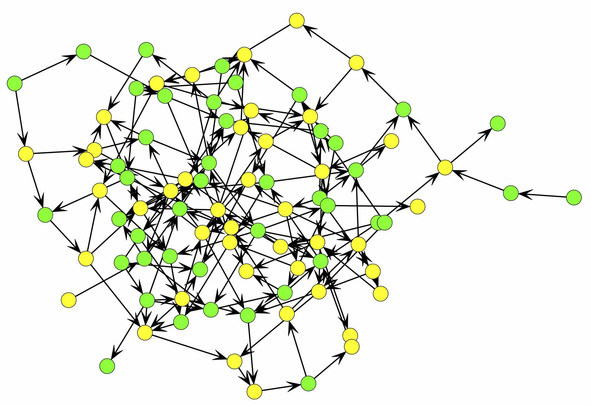
Lets generate some node colors using "Gender" again to color the nodes.

node_colors <- rep("",Clean_Data$num_nodes)
for(i in 1:Clean_Data$num_nodes){
  if(get.node.attr(net4,"Gender")[i] == "Female"){
    node_colors[i] <- "yellow"
  }else{
    node_colors[i] <- "green"
  }
}

Now we can plot our network (keeping things simple):

pdf("Network_Plot_4.pdf", # name of pdf (need to include .pdf)
    width = 20, # width of resulting pdf in inches
    height = 20 # height of resulting pdf in inches
) 
plot.network(net4, 
             vertex.col = node_colors, #just one color
             displaylabels = F, # no node names
             mode = "kamadakawai", # another layour algorithm
             displayisolates = F # remove isolate nodes from plot
)
dev.off() # finishes plotting and finalizes pdf

Now we can go look for the plot in our working directory. You should end up with a network that looks something like this:

Checking your work.

It is important to make sure that you have read in the network correctly when you are working with messy real world data. Below I provide a function that will take a random subsample of actors and edges form the final network object and print them out to the console so you can more easily spot-check your work. This is a very good practice in general, but particularly so when we are working with relational data.

Check_Network_Integrity <- function(network_object, # the network object we created
                                    n_edges_to_check = 10 # defaults to 10 edges
                                    ){
  # Make sure we are providing a network object to the function.
  if(class(network_object) != "network"){
    stop("You must provide this function with an object of class network!")
  }
  # Get network information and edges
  num_nodes <- length(network_object$val)
  edgelist <- as.matrix(network_object, matrix.type = "edgelist")
  names <- get.vertex.attribute(network_object,"vertex.names")
  # Make sure we do not ask for more edges than are in our network
  if(n_edges_to_check > length(edgelist[,1])){
    n_edges_to_check <- length(edgelist[,1])
  }
  # Select a sample of edges
  edges_to_check <- sample(x = 1:length(edgelist[,1]), 
                           size = n_edges_to_check, 
                           replace = F)
  #print out the edges to check.
  cat("Check source data file to make sure that the following edges exist:\n\n")
  for(i in 1:n_edges_to_check){
    cat(names[edgelist[edges_to_check[i],1]],"-->",names[edgelist[edges_to_check[i],2]], "\n")
  }
  cat("\nIf any of these edges do not match your source data files, there was likely a problem reading in your data and you should revisit the process.\n")
}

Now give it a try. if all went well, you are off to the races!

Check_Network_Integrity(net4)

In this case our data look alright. This will not provide proof-positive that nothing is possibly wrong, but it is a good practice and will catch errors a surprising number of times. This concludes the tutorial, but there are many more tutorials for working with network data available on the internet and I encourage you to check a few others out.

The R code for this tutorial is available here.