R Tutorial

This page contains a combination of the materials I have presented in my introductory and intermediate R workshops for the University of Massachusetts Institute for Social Science Research -- Summer Methods Summit 2015 You can email me at matthewjdenny@gmail.com or mzd5530@psu.edu if you have any questions. Before You get started coding, I suggest you check out this tutorial (particularly the part on RStudio) as I will assume you have it installed for this tutorial.

Preliminaries -- Setting Up R To Do Work

In general, when you are working with R, you will want to start with a clean slate each time, load in the data and packages that you need, and then make sure you save your output somewhere you can find it. Fortunately, R makes this pretty easy. You can begin most R scripts by clearing your workspace -- This gets rid of all of the information that was there when you started to you have a clean slate.

rm(list = ls())

Next step is to set your working directory -- This is where R goes to look for files and save stuff by default. You will need to do this for each computer you run your script file on. In RStudio, you can go to Session -> Set Working Directory -> Choose Directory and select a folder from a drop down menu. For me, this looks like:

setwd("~/Desktop")

Basic Data Structures and Operations

The first thing we might want to to in order to do some useful programming is be able to compare things. This can be done by using a comparison operator

5 < 6
5 > 6
5 == 5
5 != 6
5 <= 5

In general, R will do its best to make two quantities comparable where possible:

5345 == "5345"

However if we assign a value to a variable, then it will compare the value in the variable, so the following will return FALSE:

i <- 5
i == "i"

Whereas these lines of code will return TRUE:

i = "i"
i == "i"

Creating Data in R

The most basic thing we can do in R is assign a value to a variable (make sure there are no spaces or symbols other than . or _ in your name)

my_value <- 24

We can create a vector using the concatenation operator:

my_vector1 <- c(1,2,3,4,5,6,12345342343521)
my_vector2 <- 1:10

We can take a look at what is stored in a variable by doing one of the following:

print(my_vector2)
cat(my_vector2)

We can get the length of the vector using the length function:

length(my_vector)

The next most complicated data structure is a matrix. We can create a matrix as follows (can only hold one kind of data -- usually numbers):

my_matrix <- matrix(c(1:25),ncol=5,nrow = 5,byrow = T )

Now on to data frames (these can hold lots of different kinds of data and are what most people use to run statistical analyses. Lets make some fake data! We can start by making each variable separately before we combine them.

student_id <- c(1:10)
grades <- c("A","B","C","A","C","F","D","B","B","A")

the rep() function repeats some variable x for a specified number of times.

class <- c(rep(0,times = 5),rep(1,times = 5))
free_lunch <- rep(TRUE,times = 10)

Now we can put them together to make a data frame, but we need to use the stringsAsFactors = FALSE argument so that we do not turn our letter grades into factor variables (a kind of categorical variable that R likes but is actually a really bad idea)

data <-data.frame(student_id,grades,class,free_lunch, stringsAsFactors = FALSE)

Now we can set column names (just make sure they do not contain spaces):

colnames(data) <- c("Student_ID", "Grades","Class","Free_Lunch")

With our own dataset created, lets try searching through our data and taking some subsets. The which() function will let us identify observations that meet a certain criteria. This example also introduces the dollar sign operator which will let us access a variable in a data frame by name:

which(data$Grades == "A")

Now we can create a new dataset that only includes A or B students by saving the indexes of the A and B students and then using them to extract a subset of the total students:

A_students <- which(data$Grades == "A")
B_students <- which(data$Grades == "B")
students_for_reduced_dataset <- c(A_students,B_students)

We can then use the vector to index only the rows we want and extract them, saving them to a new object. Note that we index by [row,column] and if we leave one of these fields blank then we take the entire row (or column).

reduced_data <- data[students_for_reduced_dataset,]

When we are subsetting data, we can use the c() function to take arbitrary subsets of a matrix:

data[c(1:5,7,9),c(2,4)]

The most flexible data structure in R is list. It can store lots of pretty much anything, and can stick together other lists, matrices, vectors and values all in one place. To create an empty list, we can do the following:

my_list <- vector("list", length = 10)

Alternatively, we can create a list from objects:

my_list <- list(10, "dog",c(1:10))

We can even add a sublist to a list:

my_list <- append(my_list, list(list(27,14,"cat")))
print(my_list)

Data I/O

In this section we are going to write our school children data to a .csv file and then read the data back in to another R object. We are also going to learn how to save R objects. Make sure you do not write row names, this can really mess things up!

write.csv(x=data, file = "school_data.csv", row.names = FALSE)

Now we are going to read the data back in from a .csv. You should make sure that you specify the correct separator (the write.csv function defaults to using comma separation). I always specify stringsAsFactors = FALSE to preserve any genuine string variables I read in.

school_data <- read.csv(file = "school_data.csv", stringsAsFactors = FALSE,sep = ",")

To read and write Excel data, we will need to load in a package which will extend the functionality of R. First we need to download the package, we can either do this manually or by using the package manager in base R. You need to make sure you select dependencies = TRUE so that you download the other packages that your package depends on, otherwise it will not work! Here is the manual way:

install.packages("xlsx", dependencies = TRUE)

Now we have to actually load the package so we can use it. We do this using the library() command:

library(xlsx)

Lets try to write our school children data to an xlsx file:

write.xlsx(data, file = "school_data.xlsx", row.names=FALSE)

We can then read in our data from the excel file:

excel_school_data <- read.xlsx(file = "school_data.xlsx", sheetIndex =1, stringsAsFactors = FALSE)

As we can see, we get back the same thing!

Lets move on to Stata Data. We will need the foreign package to read in data from Stata:

install.packages("foreign", dependencies = TRUE)

Lets load the package now:

library(foreign)

Here is how we write and read data to and from .dta file:

write.dta(data,file = "school_data.dta")
stata_school_data <- read.dta(file = "school_data.dta")

R also has its own binary data type called .Rdata files. The cool thing about an Rdata file is that it can hold everything in our workspace or just a couple of things. This is a very good strategy for saving all of your files after a day of working so you can pick back up where you left off. Here is how we might save just a few objects:

save(list = c("data", "reduced_data"), file = "Two_objects.Rdata")

But we can also just save everything in memory:

save(list= ls(), file = "MyData.Rdata")

Lets test it out by clearing our whole workspace (note that if we do this we will need to reload any packages we were using manually as they do not get saved to the .Rdata file)

rm(list= ls())

Now we can load the data back in! It is good practice to set our working directory again first (remember to change this to the folder location where you downloaded the workshop materials or saved this script file!):

setwd("~/Dropbox/RA_and_Consulting_Work/ISSR_Consulting_Work/Intro_To_R")

Lets try loading in the two objects we saved:

load(file = "Two_objects.Rdata")

and now we can load in everything:

load(file = "MyData.Rdata")

We have now covered the basics of Data IO. In the section I will move on to some basic programming.

cat vs. print

One preliminary thing we will want to think about as we start doing more programming is how we want R to tell us what it is doing. As noted earlier, this can be done using either the cat or print functions. The cat function will print things without "" marks around them, which often looks nicer, but it also does not skip to a new line if you call it multiple times inside of a function (something we will get to soon) or a loop. Lets try out both:

print("Hello World")
cat("Hello World")

Now we can try them inside brackets to see how cat does not break lines:

{
    cat("Hello")
    cat("World")
}

{
    print("Hello")
    print("World")
}

So we have to manually break lines with cat() using the " " or newline symbol:

{
    cat("Hello )
    cat("World")
}

The paste() function -- generating informative messages

The paste function takes as many string, number, or variable arguments as you want and sticks them all together using a user specified separator. This can be ridiculously useful. Lets define a variable to hold the number of fingers we have:

fingers <- 8

Now lets print out how many fingers we have:

print(paste("Hello,", "I have", fingers, "Fingers", sep = " "))

Now lets separate with dashes just for fun:

print(paste("Hello,", "I have", fingers, "Fingers", sep = "-----"))

Now lets try the same thing with cat:

cat(paste("Hello,", "I have", fingers, "Fingers", sep = " "))

However, with cat, I can just skip the paste part and it will print the stuff directly:

cat("Hello,", "I have", fingers, "Fingers", sep = " ")

If we want cat to break lines while it is printing, we can also include the " " symbol at the end (or anywhere for that matter)

cat("My Grocery List:", 
"1 dozen eggs",
"1 loaf of bread",
"1 bottle of orange juice", 
"1 pint mass mocha", 
sep = " ")

For Loops

For loops are a way to automate performing tasks my telling R how many times you want to do something. Along with conditional statements and comparison operators, loops are more powerful than you can imagine. Pretty much everything on your computer can be boiled down to a combinations of these. Here is the basic syntax, with a translation to english below:

# for (           i in           1:10){
# for each number i in the range 1:10

Example of a for() loop -- first lets make a vector of data:

my_vector <- c(20:30)

We can take a look first:

cat(my_vector)

Now we can take the square root of each entry using a for loop:

for(i in 1:length(my_vector)){
    cat(i,"\n")
    my_vector[i] <- sqrt(my_vector[i])
}

and display the result:

cat(my_vector)

Lets add some stuff together:

my_num <- 0
for(i in 1:100){
    my_num <- my_num + i
    cat("Current Iteration:",i,"My_num value:",my_num,"\n")
}

If/Else Statements

These give your computer a "brain", they let it see if something is the case, and dependent on that answer your compute can then take some desired action. Here is the basic syntax, with a translation to english below:

#if(some condition is met){
#     do something
#}

Lets try an example to check and see if our number is equal to 20

my_number <- 19
if(my_number < 20){
    cat("My number is less than 20 \n")
}
my_number <- 22
if(my_number < 20){
    cat("My number is less than 20 \n")
}

Here is another example of an if statement in a for loop:

my_vector <- c(20:30)
for(i in 1:length(my_vector)){
    cat("Current Index:",i,"Value:",my_vector[i],"\n")
    if(my_vector[i] == 25){
        cat("The square root is 5! \n")
    }
}

You can also add in an else statement to do something else if the condition is not met.

my_vector <- c(20:30)
for(i in 1:length(my_vector)){
    cat("Current Index:",i,"Value:",my_vector[i],"\n")
    if(my_vector[i] == 25){
        print("I am 25!")
    }else{
        print("I am not 25!")
    }
}

Functions

User defined functions allow you to easily reuse a section of code. They are both the most powerful, and most complex tool available in the R language. Here is a basic example where we define a function that will take the sum of a particular column of a matrix (where the column index is a number).

my_column_sum <- function(col_number,my_matrix){ 
    #take the column sum of the matrix
    col_sum <- sum(my_matrix[,col_number])
    return(col_sum)
}

lets try it out:

my_mat <- matrix(1:100,nrow=10,ncol=10)

start by looking at our matrix:

my_mat

Now lets take the column sum of the first column:

temp <- my_column_sum(col_number = 1, my_matrix = my_mat)

Lets double check

sum(my_mat[,1])

Now we can loop through all columns in the matrix:

for(i in 1:10){
    cat(my_column_sum(i,my_mat),"\n")
}

A Google Scholar Web Scraper:

Now lets try a more complicated example -- write a function to go get the number of results that pop up for a given name in google scholar. First we will need to load a few packages which will help us out along the way.

install.packages("scrapeR")
install.packages("stringr")
library(scrapeR)
library(stringr)

Now we can define a function that will get the raw html of the webpage, download it, and extract what we want from it. See the inline comments for what each line of code does:

get_google_scholar_results <- function(string, return_source = FALSE){

    # print out the input name
    cat(string, "\n")
	
    # make the input name all lowercase
    string <- tolower(string)

    # split the string on spaces
    str <- str_split(string," ")[[1]]

    # combine the resulting parts of the string with + signs so "Matt Denny" will end up as "matt+denny" which is what Google Scholar wants as input
    str <- paste0(str,collapse = "+")

    # add the name (which is now in the correct format) to the search query and we have our web address.
    str <- paste("https://scholar.google.com/scholar?hl=en&q=",str,sep = "")

    # downloads the web page source code
    page <- getURL(str, .opts = list(ssl.verifypeer = FALSE))

    # search for the 'Scholar</a><div id="gs_ab_md">' string which occurs uniquely right before google Scholar tells you how many results your query returned
    num_results <- str_split(page,'Scholar</a><div id=\"gs_ab_md\">')[[1]][2]

    # split the resulting string on the fist time you see a "(" as this will signify the end of the text string telling you how many results were returned. 
    num_results <- str_split(num_results,'\(')[[1]][1]

    # Print out the number of results returned by Google Scholar
    cat("Query returned", tolower(num_results), "\n")
	
	# Look to see if the "User profiles" string is present -- grepl will return true if the specified text ("User profiles") is contained in the web page source. 
    if(grepl("User profiles",page)){

        # split the web page source (which is all one string) on the "Cited by " string and then take the second chunk of the resulting vector of substrings (so we can get at the number right after the first mention of "Cited by ")
        num_cites <- str_split(page,"Cited by ")[[1]][2]

        # now we want the number before the < symbol in the resulting string  (which will be the number of cites)
        num_cites <- str_split(num_cites,"<")[[1]][1]

        # now let the user know how many we found
        cat("Number of Cites:",num_cites,"\n")

    }else{
        # If we could not find the "User profiles" string, then the person probably does not have a profile on Google Scholar and we should let the user know this is the case
        cat("This user may not have a Google Scholar profile \n")
    }
    
	# If we specified the option at the top that we wanted to return the HTML source, then return it, otherwise don't.
    if(return_source){
        return(page) 
    }
}

Now lets have some fun...

get_google_scholar_results("William Jacoby")
get_google_scholar_results("Laurel Smith-Doerr")
get_google_scholar_results("Noam Chomsky")
get_google_scholar_results("Gary King")

One important thing to note is that you need to take it slow while web scraping. As a general rule, when you are starting out, you should limit yourself to 10 page requests a minute.

A Data Cleaning and Plotting Example

This is a little toy example reading in some data from start to finish. You can download the example data here. Once you have downloaded the data, you will need to set your working directory to the folder where you saved the data. Note that you will have to extract the zip file first. Having done so, lets read in some data:

load("Example_Data.Rdata")

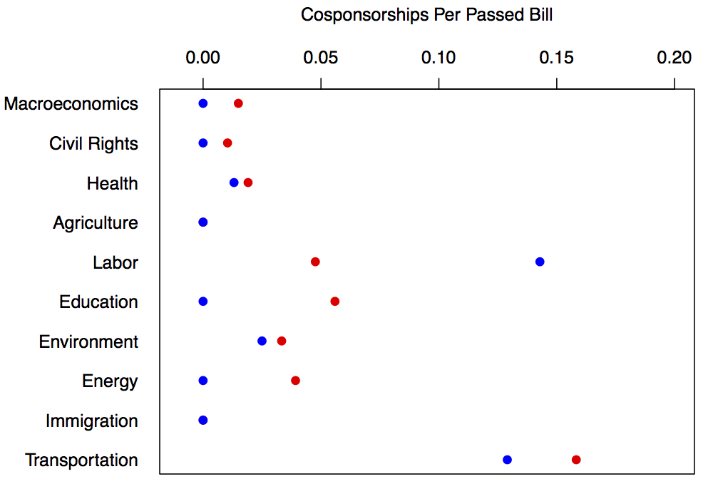
This is a dataset with metadata on all bills introduced in the United States Congress between 2011-2012 (from the Congressional Bills Project). Among many variables, it contains indicators of the number of cosponsors, the month the bill was introduced, the chamber it was introduced in (House or Senate), the major topic code (see reference list below) and the party of the sponsor. Lets say we wanted to look at a subset of all bills that were introduced in the House that were about any of the first ten topics and then take a the sum of the number of bills introduced in each category by each party that passed the house and divide by the total number of cosponsorships they received to get a weight for the "effectiveness" of each cosponsorship. Here are the topics by major topic number ---

Macroeconomics
Civil Rights, Minority Issues, and Civil Liberties
Health
Agriculture
Labor and Employment
Education
Environment
Energy
Immigration
Transportation
Law, Crime, and Family Issues
Social Welfare
Community Development and Housing Issues
Banking, Finance, and Domestic Commerce
Defense
Space, Science, Technology and Communications
Foreign Trade
International Affairs and Foreign Aid
Government Operations

Note that some of these are missing from the dataset (because they are not represented in the sample). Lets start by subsetting our data -- we only want HR bills (introduced in the House) with a major topic less than 11:

reduced_data <- data[which(data$BillType == "HR" &  data$Major < 11),]

We can now define a matrix to hold our calculated statistics:

party_monthly_statistics <- matrix(0, nrow = 10, ncol = 2)

Now we will make be putting everything together, with nested looping and conditional statements in the same chunk of code. Lets start by looping over topics:

for(i in 1:10){
    #now for each category we loop over parties
    for(j in 1:2){
        # set the variable we are going to lookup against for party ID
        if(j == 1){
            party <- 100
        }else{
            party <- 200
        }
        current_data <- reduced_data[which(reduced_data$Party == party & reduced_data$Major == i),]
        if(length(current_data[,1]) > 0){
            # Now subset to those that passed the house
            current_data <- current_data[which(current_data$PassH == 1),]
            #calculate the weight
            cosponsorship_weight <- length(current_data[,1])/sum(current_data$Cosponsr)
            #check to see if it is a valid weight, if not, set equal to zero
            if(is.nan(cosponsorship_weight) | cosponsorship_weight > 1 ){
                cosponsorship_weight <- 0
            }
            #take that weight and put it in our dataset
            party_monthly_statistics[i,j] <- cosponsorship_weight
        }
    }
}

Now lets create labels for bill major topics:

labs <- c("Macroeconomics", "Civil Rights", "Health" , "Agriculture", "Labor", "Education", "Environment", "Energy", "Immigration", Transportation")

Now it is time to plot. We are going to put everything in a PDF so we can start by specifying the dimensions of our PDF output and the title:

pdf(width = 5,height = 8, file = "My_Plot.pdf")

We want a wider margin on the bottom and left sides so our text will fit. margins go (bottom, left, top, right):

par(mar = c(13,5,2,2))

Now it is time to plot our data using matplot which lets us easily plot more than one series on the same axes:

matplot(x= 1:10,  #this tells matplot what the x values should be
        y=cbind(party_monthly_statistics[,2],party_monthly_statistics[,1]), #this reverses democrat and republican so it is easier to see the democrat points and then specifies the y values
        pch = 19, #this sets the point type to be dots 
        xlab = "", #this say do not plot an x label as we will specify it later
        ylab = "Cosponsorships Per Passed Bill", #the y label
        xaxt = "n", #don't plot any x-axis ticks 
        col = c("red","blue"), #the colors for the dots, blue is democrat, red is republican
        ylim = c(-0.01,.2) #the y-limits of the plotting range
        )

now we can add a custom x-axis with our text labels

axis(side = 1, at = 1:10, tick = FALSE, labels = labs, las = 3)

We are now done making our pdf so finalize it:

dev.off()

Now all that is left is to check out the output!

oops!

Resources

This concludes the tutorial. These are only some very basic skills. Your best bet moving forward is to try and take as much as you can from this code and adapt it to your own data management tasks. Practice makes perfect. You should also definitely check out more tutorials including but not limited to these following resources:

A nice place to start learning R interactively is Swirl.
Quick-R has a bunch of easy to read tutorials for doing all sorts of basic things -- http://www.statmethods.net/.
Hadley Wickham wrote a book that covers a bunch of advanced functionality in R, titled Advanced R -- which is available online for free here -- http://adv-r.had.co.nz/.